Custom functions for preparing data

Last week, I explained how I used a combination of macros in Google Sheets to clean up class lists for a project I’m working on.

With that part of the project complete, the next step was to combine the individual class lists into one consolidated list that I could de-duplicate (many students appear in more than one class list).

There’s a simple way to combine data from multiple sheets (tabs) in a Google Sheets workbook: the Query function works well.

Here’s the problem: There are more than 90 sheets in my workbook! To make matters worse, each sheet has a name that’s easy to read and that accurately describes the class list it contains, but that is not quick to type.

This is an example of what the Query formula would look like with two of my sheets:

=QUERY({'2004-Fall-152-01'!A2:C; '2004-Fall-152-02'!A2:C}, "where Col1 is not null", 0)

Imagine typing in more than 90 additional sheet names and ranges inside those curly brackets — no thanks!

To save myself a ton of typing and reduce the risk of inadvertently introducing errors into the formula, I knew I needed to automate the process of creating the query.

That meant creating a new function in Google Apps Script. I broke the task of building the query into four steps:

1. List the names of all relevant sheets in the workbook.
2. Add the cell range and a semicolon to each sheet name.
3. Remove the semicolon from the final sheet name in the list (to avoid a formula parse error).
4. Now that I have the information that needs to go inside the curly brackets, enclose it in the rest of the formula.

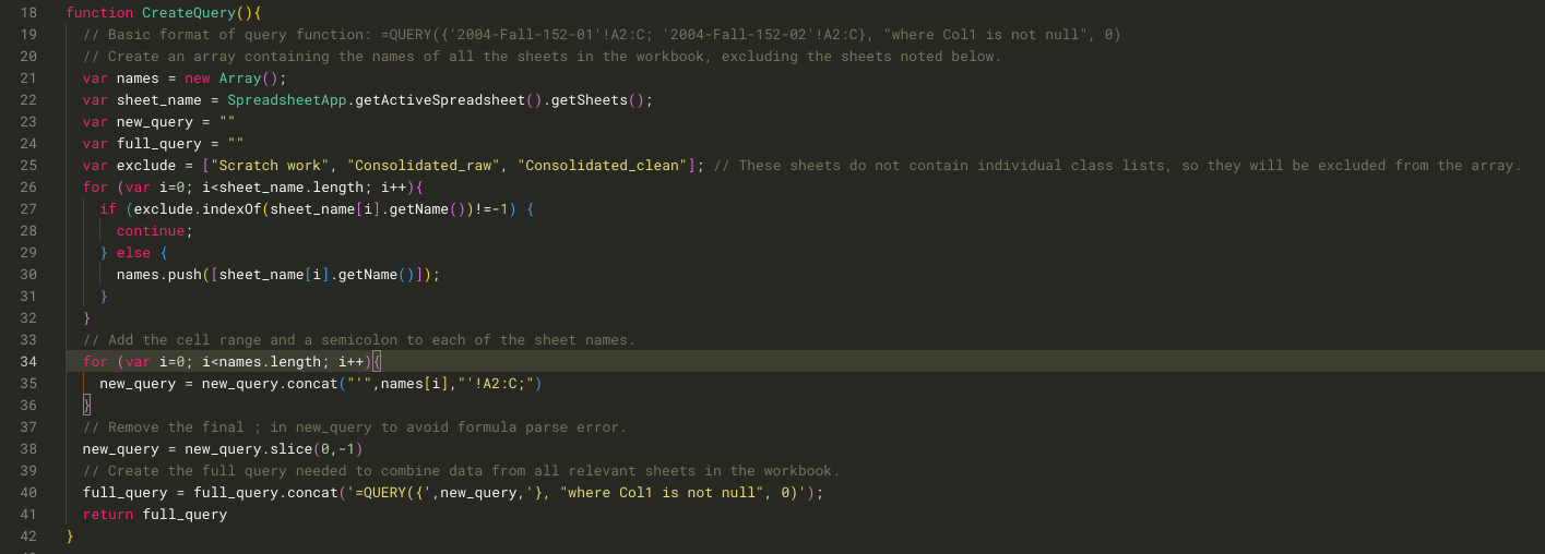
Here’s the code:

function CreateQuery(){
  // Create an array containing the names of all the sheets in the workbook, excluding the sheets noted below.
  var names = new Array();
  var sheet_name = SpreadsheetApp.getActiveSpreadsheet().getSheets();
  var new_query = ""
  var full_query = ""
  var exclude = ["Scratch work", "Consolidated_raw", "Consolidated_clean"]; // These sheets do not contain individual class lists, so they will be excluded from the array. 
  for (var i=0; i<sheet_name.length; i++){
    if (exclude.indexOf(sheet_name[i].getName())!=-1) {
      continue;
    } else {
      names.push([sheet_name[i].getName()]);
    }
  }
  // Add the cell range and a semicolon to each of the sheet names.
  for (var i=0; i<names.length; i++){
    new_query = new_query.concat("'",names[i],"'!A2:C;")
  }
  // Remove the final ; in new_query to avoid formula parse error.
  new_query = new_query.slice(0,-1)
  // Create the full query needed to combine data from all relevant sheets in the workbook.
  full_query = full_query.concat('=QUERY({',new_query,'}, "where Col1 is not null", 0)');
  return full_query
}

With that function, getting a full list of students can now be accomplished in just a few keystrokes. All I need to do is choose a blank cell, enter =CreateQuery(), and press return. That provides me with a query that I can copy and paste to get my full list of students, ready for de-duplication.